Распределение вероятностей

Распределение вероятностей — это закон, описывающий область значений случайной величины и соответствующие вероятности появления этих значений.

Определение

Пусть задано вероятностное пространство [math]\displaystyle{ (\Omega, \mathcal{F}, \mathbb{P}) }[/math], и на нём определена случайная величина [math]\displaystyle{ X:\Omega \to \mathbb{R} }[/math]. В частности, по определению, [math]\displaystyle{ X }[/math] является измеримым отображением измеримого пространства [math]\displaystyle{ (\Omega, \mathcal{F}) }[/math] в измеримое пространство [math]\displaystyle{ (\mathbb{R},\mathcal{B}(\mathbb{R})) }[/math], где [math]\displaystyle{ \mathcal{B}(\mathbb{R}) }[/math] обозначает борелевскую сигма-алгебру на [math]\displaystyle{ \mathbb{R} }[/math]. Тогда случайная величина [math]\displaystyle{ X }[/math] индуцирует вероятностную меру [math]\displaystyle{ \mathbb{P}^X }[/math] на [math]\displaystyle{ \mathbb{R} }[/math] следующим образом:

[math]\displaystyle{ \mathbb{P}^X(B) = \mathbb{P}(X^{-1}(B)),\; \forall B\in \mathcal{B}(\mathbb{R}). }[/math]

Мера [math]\displaystyle{ \mathbb{P}^X }[/math] называется распределением случайной величины [math]\displaystyle{ X }[/math]. Иными словами, [math]\displaystyle{ \mathbb{P}^X(B)=\mathbb{P}(X\in B) }[/math], таким образом [math]\displaystyle{ \mathbb{P}^X(B) }[/math] задаёт вероятность того, что случайная величина [math]\displaystyle{ X }[/math] попадает во множество [math]\displaystyle{ B\in \mathcal{B}(\mathbb{R}) }[/math].

Примеры и применение

Для дискретной случайной величины распределение вероятностей отображается как последовательность значений случайной величины и соответствующих им вероятностей. Так, для примера с игральными костями (См. Случайная_величина#Бросание_игральных_костей) распределение вероятностей будет отображаться как таблица (См. рисунок).

• Пример случайной величины и ее распределения вероятностей
• 

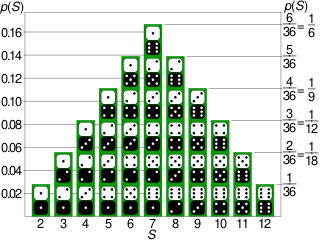
  Если пространство исходов равно множеству всех возможных комбинаций очков на двух костях, и случайная величина равна сумме этих очков, тогда S — дискретная случайная величина, чьё распределение описывается функцией вероятности, значение которой изображено как высота соответствующей колонки.

• 

  Распределение вероятностей для исходов бросания двух костей

Также распределение вероятностей может отображаться как формула, позволяющая находить вероятность любого значения случайной величины.

Для непрерывной случайной величины такой подход неприменим, поскольку, во-первых, значений случайной величины несчетное множество и, во-вторых, значение вероятности для каждого отдельно взятого значения случайной величины равно нулю.

Классификация распределений

Функция [math]\displaystyle{ F_X(x) = \mathbb{P}^X((-\infty,x]) = \mathbb{P}(X \leqslant x) }[/math] называется (кумулятивной) функцией распределения случайной величины [math]\displaystyle{ X }[/math]. Из свойств вероятности вытекает теорема:

Функция распределения [math]\displaystyle{ F_X(x) }[/math] любой случайной величины удовлетворяет следующим трем свойствам:

1. [math]\displaystyle{ F_X }[/math] — функция неубывающая;
2. [math]\displaystyle{ \lim_{x\to -\infty} F_X(x) = 0,\; \lim_{x\to \infty}F_X(x) = 1 }[/math];
3. [math]\displaystyle{ F_X }[/math] непрерывна справа.

Из того факта, что борелевская сигма-алгебра на вещественной прямой порождается семейством интервалов вида [math]\displaystyle{ \{(-\infty,x]\}_{x\in \mathbb{R}} }[/math], вытекает теорема:

Любая функция [math]\displaystyle{ F(x) }[/math], удовлетворяющая трём свойствам, перечисленным выше, является функцией распределения для какого-то распределения [math]\displaystyle{ \mathbb{P}^X }[/math].

Для вероятностных распределений, обладающих определенными свойствами, существуют более удобные способы их задания. В то же время распределения (и случайные величины) принято классифицировать по характеру функций распределения.

Дискретные распределения

Случайная величина [math]\displaystyle{ X }[/math] называется простой или дискретной, если она принимает не более, чем счётное число значений. То есть [math]\displaystyle{ X(\omega) = a_i,\; \forall \omega \in A_i }[/math], где [math]\displaystyle{ \{A_i\}_{i=1}^{\infty} }[/math] — разбиение [math]\displaystyle{ \Omega }[/math].

Распределение простой случайной величины тогда по определению задаётся: [math]\displaystyle{ \mathbb{P}^X(B) = \sum_{i:a_i \in B} \mathbb{P}(A_i) }[/math]. Введя обозначение [math]\displaystyle{ p_i = \mathbb{P}(A_i) }[/math], можно задать функцию [math]\displaystyle{ p(a_i) = p_i }[/math]. В силу свойств вероятности [math]\displaystyle{ \sum_{i=1}^{\infty}p_i = 1 }[/math]. Используя счётную аддитивность [math]\displaystyle{ \mathbb{P} }[/math], легко показать, что эта функция однозначно определяет распределение [math]\displaystyle{ X }[/math].

Набор вероятностей [math]\displaystyle{ p(a_i) = p_i }[/math], где [math]\displaystyle{ \sum_{i=1}^{\infty} p_i = 1 }[/math] называется распределением вероятностей дискретной случайной величины [math]\displaystyle{ X }[/math]. Совокупность значений [math]\displaystyle{ a_i, i=1,2... \infty }[/math] и вероятностей [math]\displaystyle{ p_i, i \in {1,2... \infty} }[/math] называется дискретным законом распределения вероятностей.

Для иллюстрации сказанного выше, рассмотрим следующий пример.

Пусть функция [math]\displaystyle{ p }[/math] задана таким образом, что [math]\displaystyle{ p(-1) = \frac{1}{2} }[/math] и [math]\displaystyle{ p(1) = \frac{1}{2} }[/math]. Эта функция задаёт распределение случайной величины [math]\displaystyle{ X }[/math], для которой [math]\displaystyle{ \mathbb{P}(X=\pm 1) = \frac{1}{2} }[/math] (см. распределение Бернулли, где случайная величина принимает значения [math]\displaystyle{ 0,1 }[/math]). Случайная величина [math]\displaystyle{ X }[/math] является моделью подбрасывания уравновешенной монеты.

Другими примерами дискретных случайных величин являются распределение Пуассона, биномиальное распределение, геометрическое распределение.

Дискретное распределение обладает следующими свойствами:

1. [math]\displaystyle{ p_i \geqslant 0 }[/math],
2. [math]\displaystyle{ \sum_{i=1}^{n} p_i = 1 }[/math], если множество значений - конечное — из свойств вероятности,
3. Функция распределения [math]\displaystyle{ F_X(x) }[/math] имеет конечное или счётное множество точек разрыва первого рода,
4. Если [math]\displaystyle{ x_0 }[/math] - точка непрерывности [math]\displaystyle{ F_X(x) }[/math], то существует [math]\displaystyle{ \frac{d F_X(x_0)}{dx}=0 }[/math].

Решётчатые распределения

Решётчатым называется распределение с дискретной функцией распределения и точки разрыва функции распределения образуют подмножество точек вида [math]\displaystyle{ a+nh }[/math], где [math]\displaystyle{ a }[/math] - вещественное, [math]\displaystyle{ h \gt 0 }[/math], [math]\displaystyle{ n }[/math] - целое.

Теорема. Для того, чтобы функция распределения [math]\displaystyle{ F }[/math] была решётчатой с шагом [math]\displaystyle{ h }[/math], необходимо и достаточно, чтобы её характеристическая функция [math]\displaystyle{ f }[/math] удовлетворяла соотношению [math]\displaystyle{ |f(2 \pi/h)|=1 }[/math].

Абсолютно непрерывные распределения

Основная статья: Плотность вероятности

Распределение случайной величины [math]\displaystyle{ X }[/math] называется абсолютно непрерывным, если существует неотрицательная функция [math]\displaystyle{ f_X:\mathbb{R}\to \mathbb{R}_+ }[/math], такая что [math]\displaystyle{ \mathbb{P}^X(B) \equiv \mathbb{P}(X\in B) = \int\limits_B f_X(x)\, dx }[/math]. Функция [math]\displaystyle{ f_X }[/math] тогда называется плотностью распределения вероятностей случайной величины [math]\displaystyle{ X }[/math]. Функция таких распределений абсолютно непрерывна в смысле Лебега.

Примерами абсолютно непрерывных распределений являются нормальное распределение, равномерное распределение, экспоненциальное распределение, распределение Коши.

Пример. Пусть [math]\displaystyle{ f(x) = 1 }[/math], когда [math]\displaystyle{ 0\leqslant x \leqslant 1 }[/math], и [math]\displaystyle{ f(x) = 0 }[/math] в противном случае. Тогда [math]\displaystyle{ \mathbb{P}(a \lt X \lt b) = \int\limits_a^b 1\, dx = b-a }[/math], если [math]\displaystyle{ (a,b) \subset [0,1] }[/math].

Для любой плотности распределения [math]\displaystyle{ f_X }[/math] верны свойства:

1. [math]\displaystyle{ f_X(x) \geqslant 0 }[/math];
2. [math]\displaystyle{ \int\limits_{-\infty}^{\infty} f_X(x)\, dx = 1 }[/math].

Верно и обратное — если функция [math]\displaystyle{ f:\mathbb{R}\to \mathbb{R} }[/math] такая, что:

1. [math]\displaystyle{ f(x) \geqslant 0,\; \forall x \in \mathbb{R} }[/math];
2. [math]\displaystyle{ \int\limits_{-\infty}^{\infty} f(x)\, dx = 1 }[/math],

то существует распределение [math]\displaystyle{ \mathbb{P}^X }[/math] такое, что [math]\displaystyle{ f(x) }[/math] является его плотностью.

Применение формулы Ньютона-Лейбница приводит к следующим соотношениям между функцией и плотностью абсолютно непрерывного распределения:

[math]\displaystyle{ \mathbb{P}(a \lt X \lt b) = F(b) - F(a) = \int\limits_a^b f(t)\, dt }[/math].

Теорема. Если [math]\displaystyle{ f(x) }[/math] — непрерывная плотность распределения, а [math]\displaystyle{ F(x) }[/math] — его функция распределения, то

1. [math]\displaystyle{ F'(x) = f(x),\; \forall x \in \mathbb{R}, }[/math]
2. [math]\displaystyle{ F(x) = \int\limits_{-\infty}^x f(t)\, dt }[/math].

При построении распределения по эмпирическим (опытным) данным следует избегать ошибок округления.

Сингулярные распределения

Основная статья: Сингулярное распределение

Кроме дискретных и непрерывных случайных величин существуют величины, не являющиеся ни на одном интервале ни дискретными, ни непрерывными. К таким случайным величинам относятся, например, те, функции распределения которых непрерывные, но возрастают только на множестве лебеговой меры нуль.

Сингулярными называют распределения, сосредоточенные на множестве нулевой меры (обычно меры Лебега).

Таблица основных распределений

Дискретные распределения

Название	Обозначение	Параметр	Носитель	Плотность (последовательность вероятностей)	Матем. ожидание	Дисперсия	Характеристическая функция
Дискретное равномерное	[math]\displaystyle{ \text{R}\{1, \dots, N\} }[/math]	[math]\displaystyle{ N \in \mathbb N }[/math]	[math]\displaystyle{ \{1, \dots, N\} }[/math]	[math]\displaystyle{ \mathrm P(\{k\}) = \frac{1}{N}, k \in \{1, \dots, N\} }[/math]	[math]\displaystyle{ \frac{N+1}{2} }[/math]	[math]\displaystyle{ \frac{N^2 - 1}{12} }[/math]	[math]\displaystyle{ \frac{e^{it} - e^{i(N+1)t}}{N(1-e^{it})} }[/math]
Бернулли	[math]\displaystyle{ \text{Bern}(p) }[/math]	[math]\displaystyle{ p \in (0, 1) }[/math]	[math]\displaystyle{ \{0, 1\} }[/math]	[math]\displaystyle{ \mathrm P(\{0\}) = 1 - p, \mathrm P(\{1\}) = p }[/math]	[math]\displaystyle{ p }[/math]	[math]\displaystyle{ p(1-p) }[/math]	[math]\displaystyle{ pe^{it}+1-p }[/math]
Биномиальное	[math]\displaystyle{ \text{Bin}(n, p) }[/math]	[math]\displaystyle{ n \in \mathbb N, p \in (0, 1) }[/math]	[math]\displaystyle{ \{0, \dots, n\} }[/math]	[math]\displaystyle{ \mathrm P(\{k\}) = C_n^kp^k(1-p)^{n-k} }[/math]	[math]\displaystyle{ np }[/math]	[math]\displaystyle{ np(1-p) }[/math]	[math]\displaystyle{ (pe^{it}+1-p)^n }[/math]
Пуассоновское	[math]\displaystyle{ \text{Pois}(\lambda) }[/math]	[math]\displaystyle{ \lambda \gt 0 }[/math]	[math]\displaystyle{ \mathbb Z_+ }[/math]	[math]\displaystyle{ \mathrm P(\{k\}) = \frac{\lambda^k}{k!}e^{-\lambda} }[/math]	[math]\displaystyle{ \lambda }[/math]	[math]\displaystyle{ \lambda }[/math]	[math]\displaystyle{ e^{\lambda(e^{it} - 1)} }[/math]
Геометрическое	[math]\displaystyle{ \text{Geom}(p) }[/math]	[math]\displaystyle{ p \in (0, 1] }[/math]	[math]\displaystyle{ \mathbb N }[/math]	[math]\displaystyle{ \mathrm P (\{k\}) = (1 - p)^{k-1}p }[/math]	[math]\displaystyle{ \frac{1}{p} }[/math]	[math]\displaystyle{ \frac{1-p}{p^2} }[/math]	[math]\displaystyle{ \frac{pe^{it}}{1 - (1-p)e^{it}} }[/math]

Абсолютно непрерывные распределения

Название	Обозначение	Параметр	Носитель	Плотность вероятности [math]\displaystyle{ f(x) }[/math]	Функция распределения F(х)	Характеристическая функция	Математическое ожидание	Медиана	Мода	Дисперсия	Коэффициент асимметрии	Коэффициент эксцесса	Дифференциальная энтропия	Производящая функция моментов
Равномерное непрерывное	[math]\displaystyle{ U(a, b) }[/math]	[math]\displaystyle{ a, b \in \mathbb R, a \lt b }[/math], [math]\displaystyle{ a }[/math] — коэффициент сдвига, [math]\displaystyle{ b-a }[/math] — коэффициент масштаба	[math]\displaystyle{ [a, b] }[/math]	[math]\displaystyle{ \dfrac{1}{b-a}I\{x \in [a, b]\} }[/math]	[math]\displaystyle{ \dfrac{x-a}{b-a}I\{x \in [a, b]\} + I\{x \gt b\} }[/math]	[math]\displaystyle{ \dfrac{e^{itb} - e^{ita}}{it(b-a)} }[/math]	[math]\displaystyle{ \frac{a+b}{2} }[/math]	[math]\displaystyle{ \frac{a+b}{2} }[/math]	любое число из отрезка [math]\displaystyle{ [a,b] }[/math]	[math]\displaystyle{ \frac{(b-a)^2}{12} }[/math]	[math]\displaystyle{ 0 }[/math]	[math]\displaystyle{ -\frac{6}{5} }[/math]	[math]\displaystyle{ \ln(b-a) }[/math]	[math]\displaystyle{ \frac{e^{tb}-e^{ta}}{t(b-a)} }[/math]
Нормальное (гауссовское)	[math]\displaystyle{ N(\mu, \sigma^2) }[/math]	[math]\displaystyle{ \mu \in \mathbb R }[/math]— коэффициент сдвига, [math]\displaystyle{ \sigma \gt 0 }[/math] — коэффициент масштаба	[math]\displaystyle{ \mathbb R }[/math]	[math]\displaystyle{ \frac{1}{\sigma\sqrt{2\pi}}\; e^{-\frac{\left(x-\mu\right)^2}{2\sigma^2}} }[/math]	[math]\displaystyle{ \frac{1}{2} \left( 1 + \operatorname{erf} \left( \frac{x-\mu}{\sqrt{2\sigma^2}} \right) \right) }[/math]	[math]\displaystyle{ e^{i\,\mu\,t-\frac{\sigma^2 t^2}{2}} }[/math]	[math]\displaystyle{ \mu }[/math]	[math]\displaystyle{ \mu }[/math]	[math]\displaystyle{ \mu }[/math]	[math]\displaystyle{ \sigma^2 }[/math]	[math]\displaystyle{ 0 }[/math]	[math]\displaystyle{ 0 }[/math]	[math]\displaystyle{ \ln\left(\sigma\sqrt{2\,\pi\,e}\right) }[/math]	[math]\displaystyle{ e^{\mu\,t+\frac{\sigma^2 t^2}{2}} }[/math]
Логнормальное	[math]\displaystyle{ LN(\mu,\sigma^2) }[/math]	[math]\displaystyle{ \mu \in \mathbb R, \sigma \gt 0 }[/math]	[math]\displaystyle{ (0; +\infty) }[/math]	[math]\displaystyle{ \frac{1}{x\sigma\sqrt{2\pi}}e^{-\frac{1}{2}\left(\frac{\ln(x)-\mu}{\sigma}\right)^2} }[/math]	[math]\displaystyle{ \frac{1}{2}+\frac{1}{2} \mathrm{Erf}\left[\frac{\ln(x)-\mu}{\sigma\sqrt{2}}\right] }[/math]	[math]\displaystyle{ \sum_{n=0}^{\infty}\frac{(it)^n}{n!}e^{n\mu+n^2\sigma^2/2} }[/math]	[math]\displaystyle{ e^{\mu+\sigma^2/2} }[/math]	[math]\displaystyle{ e^{\mu} }[/math]	[math]\displaystyle{ e^{\mu-\sigma^2} }[/math]	[math]\displaystyle{ (e^{\sigma^2}\!\!-1) e^{2\mu+\sigma^2} }[/math]	[math]\displaystyle{ (e^{\sigma^2}\!\!+2)\sqrt{e^{\sigma^2}\!\!-1} }[/math]	[math]\displaystyle{ e^{4\sigma^2}\!\!+2e^{3\sigma^2}\!\!+3e^{2\sigma^2}\!\!-6 }[/math]	[math]\displaystyle{ \frac{1}{2}+\frac{1}{2}\ln(2\pi\sigma^2) + \mu }[/math]	[math]\displaystyle{ e^{s\mu + \tfrac{1}{2}s^2\sigma^2}. }[/math]
Гамма-распределение	[math]\displaystyle{ \Gamma(\alpha, \beta) }[/math]	[math]\displaystyle{ \alpha \gt 0, \beta \gt 0 }[/math]	[math]\displaystyle{ \mathbb R_+ }[/math]	[math]\displaystyle{ \frac{\alpha^{\beta}x^{\beta - 1}}{\Gamma(\beta)}e^{-\alpha x} }[/math]	[math]\displaystyle{ \frac{1}{\Gamma(\beta)} \gamma(\beta, \alpha x) }[/math]	[math]\displaystyle{ \left(1 - \frac{it}{\alpha}\right)^{-\beta} }[/math]	[math]\displaystyle{ \frac{\beta}{\alpha} }[/math]		[math]\displaystyle{ \frac{\beta - 1}{\alpha} }[/math] при [math]\displaystyle{ \beta \geq 1 }[/math]	[math]\displaystyle{ \frac{\beta}{\alpha^2} }[/math]	[math]\displaystyle{ \frac{2}{\sqrt{\beta}} }[/math]	[math]\displaystyle{ \frac{6}{\beta} }[/math]	[math]\displaystyle{ \begin{align} \beta &- \ln \alpha + \ln\Gamma(\beta)\\ &+ (1 - \beta)\psi(\beta) \end{align} }[/math]	[math]\displaystyle{ \left(1 - \frac{t}{\alpha}\right)^{-\beta} }[/math] при [math]\displaystyle{ t \lt \alpha }[/math]
Экспоненциальное	[math]\displaystyle{ \text{Exp}(\lambda) }[/math]	[math]\displaystyle{ \lambda \gt 0 }[/math]	[math]\displaystyle{ \mathbb R_+ }[/math]	[math]\displaystyle{ \lambda e^{-\lambda x}I\{x \gt 0\} }[/math]	[math]\displaystyle{ 1 - e^{-\lambda x} }[/math]	[math]\displaystyle{ \frac{\lambda}{\lambda - it} }[/math]	[math]\displaystyle{ \frac{1}{\lambda} }[/math]	[math]\displaystyle{ \ln(2)/\lambda }[/math]	[math]\displaystyle{ 0 }[/math]	[math]\displaystyle{ \lambda^{-2} }[/math]	[math]\displaystyle{ 2 }[/math]	[math]\displaystyle{ 6 }[/math]	[math]\displaystyle{ 1 - \ln(\lambda) }[/math]	[math]\displaystyle{ \left(1 - \frac{t}{\lambda}\right)^{-1} }[/math]
Лапласа	[math]\displaystyle{ \text{Laplace}(\alpha,\beta) }[/math]	[math]\displaystyle{ \alpha\gt 0 }[/math] — коэффициент масштаба, [math]\displaystyle{ \beta\in\mathbb{R} }[/math] — коэффициент сдвига	[math]\displaystyle{ \mathbb R }[/math]	[math]\displaystyle{ \frac{\alpha}{2}\,e^{-\alpha|x-\beta|} }[/math]	[math]\displaystyle{ \begin{cases}\frac{1}{2}e^{\alpha(x-\beta)}, & x\leqslant\beta \\ 1-\frac{1}{2}e^{-\alpha(x-\beta)}, & x\gt \beta \end{cases} }[/math]	[math]\displaystyle{ \frac{\alpha^{2}}{\alpha^{2}+t^{2}}e^{it\beta} }[/math]	[math]\displaystyle{ \beta }[/math]	[math]\displaystyle{ \beta }[/math]	[math]\displaystyle{ \beta }[/math]	[math]\displaystyle{ \frac{2}{\alpha^{2}} }[/math]	[math]\displaystyle{ 0 }[/math]	[math]\displaystyle{ 3 }[/math]	[math]\displaystyle{ \ln\frac{2e}{\alpha} }[/math]	[math]\displaystyle{ \frac{e^{\beta t}}{1-\alpha^2 t^2} \text{ для }|t| \lt 1/\alpha }[/math]
Коши	[math]\displaystyle{ \text{Cauchy}(x_0, \gamma) }[/math]	[math]\displaystyle{ x_0 }[/math] — коэффициент сдвига, [math]\displaystyle{ \gamma \gt 0 }[/math] — коэффициент масштаба	[math]\displaystyle{ \mathbb R }[/math]	[math]\displaystyle{ { 1 \over \pi } \left( { \gamma \over \gamma^2 + (x - x_0)^2} \right) }[/math]	[math]\displaystyle{ \frac{1}{\pi} \mathrm{arctg}\left(\frac{x-x_0}{\gamma}\right)+\frac{1}{2} }[/math]	[math]\displaystyle{ e^{i\,x_0\,t-\gamma\,|t|} }[/math]	нет	[math]\displaystyle{ x_0 }[/math]	[math]\displaystyle{ x_0 }[/math]	[math]\displaystyle{ +\infty }[/math]	нет	нет	[math]\displaystyle{ \ln(4\,\pi\,\gamma) }[/math]	нет
Бета-распределение	[math]\displaystyle{ \text{Beta}(\alpha, \beta) }[/math]	[math]\displaystyle{ \alpha \gt 0, \beta \gt 0 }[/math]	[math]\displaystyle{ [0, 1] }[/math]	[math]\displaystyle{ \frac{x^{\alpha - 1}(1-x)^{\beta-1}}{\text{B}(\alpha, \beta)} }[/math]	[math]\displaystyle{ I_x(\alpha,\beta) }[/math]	[math]\displaystyle{ {}_1F_1(\alpha; \alpha+\beta; i\,t) }[/math]	[math]\displaystyle{ \frac{\alpha}{\alpha + \beta} }[/math]	[math]\displaystyle{ I_{\frac{1}{2}}^{[-1]}(\alpha,\beta)\approx \frac{ \alpha - \tfrac{1}{3} }{ \alpha + \beta - \tfrac{2}{3} } }[/math] для [math]\displaystyle{ \alpha, \beta \gt 1 }[/math]	[math]\displaystyle{ \frac{\alpha-1}{\alpha+\beta-2} }[/math] для [math]\displaystyle{ \alpha\gt 1, \beta\gt 1 }[/math]	[math]\displaystyle{ \frac{\alpha\beta}{(\alpha+\beta)^2(\alpha+\beta+1)} }[/math]	[math]\displaystyle{ \frac{2\,(\beta-\alpha)\sqrt{\alpha+\beta+1}}{(\alpha+\beta+2)\sqrt{\alpha\beta}} }[/math]	[math]\displaystyle{ 6\,\frac{\alpha^3-\alpha^2(2\beta-1)+\beta^2(\beta+1)-2\alpha\beta(\beta+2)}{\alpha \beta (\alpha+\beta+2) (\alpha+\beta+3)} }[/math]		[math]\displaystyle{ 1 +\sum_{k=1}^{\infty} \left( \prod_{r=0}^{k-1} \frac{\alpha+r}{\alpha+\beta+r} \right) \frac{t^k}{k!} }[/math]
хи-квадрат	[math]\displaystyle{ \chi^2(k) }[/math]	[math]\displaystyle{ k \gt 0 }[/math]— число степеней свободы	[math]\displaystyle{ \mathbb R_+ }[/math]	[math]\displaystyle{ \frac{(1/2)^{k/2}}{\Gamma(k/2)} x^{k/2 - 1} e^{-x/2} }[/math]	[math]\displaystyle{ \frac{\gamma(k/2,x/2)}{\Gamma(k/2)} }[/math]	[math]\displaystyle{ (1-2\,i\,t)^{-k/2} }[/math]	[math]\displaystyle{ k }[/math]	примерно [math]\displaystyle{ k-2/3 }[/math]	[math]\displaystyle{ k-2 }[/math] если [math]\displaystyle{ k\geq 2 }[/math]	[math]\displaystyle{ 2\,k }[/math]	[math]\displaystyle{ \sqrt{8/k} }[/math]	[math]\displaystyle{ 12/k }[/math]	[math]\displaystyle{ \frac{k}{2}\!+\!\ln\left[2\Gamma\left({k \over 2}\right)\right]\!+\!\left(1\!-\!\frac{k}{2}\right)\psi\left(\frac{k}{2}\right) }[/math]	[math]\displaystyle{ (1-2\,t)^{-k/2} }[/math], если [math]\displaystyle{ 2\,t\lt 1 }[/math]
Стьюдента	[math]\displaystyle{ \text{t}(n) }[/math]	[math]\displaystyle{ n \gt 0 }[/math] — число степеней свободы	[math]\displaystyle{ \mathbb R }[/math]	[math]\displaystyle{ \frac{\Gamma(\frac{n+1}2)} {\sqrt{n\pi}\,\Gamma(\frac{n}2)}(1+\frac{x^2}n)^{-\frac{n+1}2} }[/math]	[math]\displaystyle{ \frac{1}{2} + {x \Gamma \left( \frac{n+1}2 \right)}\frac{\,_2F_1 \left ( \frac{1}{2},\frac{n+1}2;\frac{3}{2};-\frac{x^2}{n} \right)} {\sqrt{\pi n}\,\Gamma (\frac{n}2)} }[/math]	[math]\displaystyle{ \frac{K_{n/2} \left(\sqrt{n}|t|\right) \cdot \left(\sqrt{n}|t| \right)^{n/2}} {\Gamma(n/2)2^{n/2-1}} }[/math] для [math]\displaystyle{ n \gt 0 }[/math]	[math]\displaystyle{ 0 }[/math], если [math]\displaystyle{ n\gt 1 }[/math]	[math]\displaystyle{ 0 }[/math]	[math]\displaystyle{ 0 }[/math]	[math]\displaystyle{ \frac{n}{n-2} }[/math], если [math]\displaystyle{ n\gt 2 }[/math]	[math]\displaystyle{ 0 }[/math], если [math]\displaystyle{ n\gt 3 }[/math]	[math]\displaystyle{ \frac{6}{n-4} }[/math], если [math]\displaystyle{ n\gt 4 }[/math]	[math]\displaystyle{ \begin{matrix} \frac{n+1}{2}\left[ \psi(\frac{1+n}{2}) - \psi(\frac{n}{2}) \right] \\[0.5em] + \log{\left[\sqrt{n}B(\frac{n}{2},\frac{1}{2})\right]} \end{matrix} }[/math]	Нет
Фишера	[math]\displaystyle{ F(d_1,d_2) }[/math]	[math]\displaystyle{ d_1 \gt 0,\ d_2 \gt 0 }[/math] - числа степеней свободы	[math]\displaystyle{ \mathbb R_+ }[/math]	[math]\displaystyle{ \frac{\sqrt{\frac{(d_1\,x)^{d_1}\,\,d_2^{d_2}}{(d_1\,x+d_2)^{d_1+d_2}}}}{x\,\mathrm{B}\!\left(\frac{d_1}{2},\frac{d_2}{2}\right)} }[/math]	[math]\displaystyle{ I_{\frac{d_1 x}{d_1 x + d_2}}(d_1/2, d_2/2) }[/math]	[math]\displaystyle{ \frac{\Gamma(\frac{d_1+d_2}{2})}{\Gamma(\tfrac{d_2}{2})} U \! \left(\frac{d_1}{2},1-\frac{d_2}{2},-\frac{d_2}{d_1} \imath s \right) }[/math]	[math]\displaystyle{ \frac{d_2}{d_2-2} }[/math], если [math]\displaystyle{ d_2 \gt 2 }[/math]		[math]\displaystyle{ \frac{d_1-2}{d_1}\;\frac{d_2}{d_2+2} }[/math], если [math]\displaystyle{ d_1 \gt 2 }[/math]	[math]\displaystyle{ \frac{2\,d_2^2\,(d_1+d_2-2)}{d_1 (d_2-2)^2 (d_2-4)}, }[/math] если [math]\displaystyle{ d_2 \gt 4 }[/math]	[math]\displaystyle{ \frac{(2 d_1 + d_2 - 2) \sqrt{8 (d_2-4)}}{(d_2-6) \sqrt{d_1 (d_1 + d_2 -2)}}, }[/math] если [math]\displaystyle{ d_2 \gt 6 }[/math]	[math]\displaystyle{ 12\frac{d_1(5d_2-22)(d_1+d_2-2)+(d_2-4)(d_2-2)^2}{d_1(d_2-6)(d_2-8)(d_1+d_2-2)} }[/math]	[math]\displaystyle{ \ln \Gamma \left(\tfrac{d_1}{2} \right) + \ln \Gamma \left(\tfrac{d_2}{2} \right) - \ln \Gamma \left(\tfrac{d_1+d_2}{2} \right) + \! }[/math] [math]\displaystyle{ \left(1-\tfrac{d_1}{2} \right) \psi \left(1+\tfrac{d_1}{2} \right) - \left(1+\tfrac{d_2}{2} \right) \psi \left(1+\tfrac{d_2}{2} \right) \! }[/math] [math]\displaystyle{ + \left(\tfrac{d_1 + d_2}{2} \right) \psi \left(\tfrac{d_1 + d_2}{2} \right) + \ln \frac{d_1}{d_2} \! }[/math]
Рэлея	[math]\displaystyle{ \mathrm{Rayleigh}(\sigma) }[/math]	[math]\displaystyle{ \sigma }[/math]	[math]\displaystyle{ \mathbb R_+ }[/math]	[math]\displaystyle{ \frac{x}{{{\sigma }^{2}}}e^{-\frac{{{x}^{2}}}{2{{\sigma }^{2}}}} }[/math]	[math]\displaystyle{ 1-e^{\frac{-x^2}{2\sigma^2}} }[/math]	[math]\displaystyle{ 1\!-\!\sigma te^{-\sigma^2t^2/2}\sqrt{\frac{\pi}{2}}\!\left(\textrm{erfi}\!\left(\frac{\sigma t}{\sqrt{2}}\right)\!-\!i\right) }[/math]	[math]\displaystyle{ \sqrt{\frac{\pi}{2}} \sigma }[/math]	[math]\displaystyle{ \sigma\sqrt{\ln(4)} }[/math]	[math]\displaystyle{ \sigma }[/math]	[math]\displaystyle{ \left( 2-\pi /2 \right){{\sigma }^{2}} }[/math]	[math]\displaystyle{ \frac{2\sqrt{\pi}(\pi - 3)}{(4-\pi)^{3/2}} }[/math]	[math]\displaystyle{ -\frac{6\pi^2 - 24\pi +16}{(4-\pi)^2} }[/math]	[math]\displaystyle{ 1+\ln\left(\frac{\sigma}{\sqrt{2}}\right)+\frac{\gamma}{2} }[/math]	[math]\displaystyle{ 1+\sigma t\,e^{\sigma^2t^2/2}\sqrt{\frac{\pi}{2}}\left(\textrm{erf}\left(\frac{\sigma t}{\sqrt{2}}\right)\!+\!1\right) }[/math]
Вейбулла	[math]\displaystyle{ \mathrm{W}(k,\lambda) }[/math]	[math]\displaystyle{ \lambda\gt 0 }[/math] - коэффициент масштаба, [math]\displaystyle{ k\gt 0 }[/math] - коэффициент формы	[math]\displaystyle{ \mathbb R_+ }[/math]	[math]\displaystyle{ \frac{k}{\lambda} \left(\frac{x}{\lambda}\right)^{k-1} e^{-\left(\frac{x}{\lambda}\right)^k} }[/math]	[math]\displaystyle{ 1- e^{-\left(\frac{x}{\lambda}\right)^k} }[/math]	[math]\displaystyle{ \sum_{n=0}^\infty \frac{(it)^n\lambda^n}{n!}\Gamma(1+n/k) }[/math]	[math]\displaystyle{ \lambda \Gamma\left(1+\frac{1}{k}\right) }[/math]	[math]\displaystyle{ \lambda\ln(2)^{1/k} }[/math]	[math]\displaystyle{ \frac{\lambda(k-1)^{\frac{1}{k}}}{k^{\frac{1}{k}}}, }[/math] для [math]\displaystyle{ k\gt 1 }[/math]	[math]\displaystyle{ \lambda^2\Gamma\left(1+\frac{2}{k}\right) - \mu^2 }[/math]	[math]\displaystyle{ \frac{\Gamma(1+\frac{3}{k})\lambda^3-3\mu\Gamma(1+\frac{2}{k})\lambda^2+2\mu^3}{\sigma^3} }[/math]	[math]\displaystyle{ \frac{\lambda^4\Gamma\left(1+\frac4k\right)-4\lambda^3\mu\Gamma\left(1+\frac3k\right)+6\lambda^2\mu^2\Gamma\left(1+\frac2k\right)-3\mu^4}{\sigma^4} }[/math]	[math]\displaystyle{ \gamma\left(1\!-\!\frac{1}{k}\right)+\left(\frac{\lambda}{k}\right)^k +\ln\left(\frac{\lambda}{k}\right) }[/math]	[math]\displaystyle{ \sum_{n=0}^\infty \frac{t^n\lambda^n}{n!}\Gamma(1+n/k), \ k\geq1 }[/math]
Логистическое	[math]\displaystyle{ L(\mu,s) }[/math]	[math]\displaystyle{ \mu }[/math], [math]\displaystyle{ s\gt 0 }[/math]	[math]\displaystyle{ \mathbb R }[/math]	[math]\displaystyle{ \frac{e^{-(x-\mu)/s}} {s\left(1+e^{-(x-\mu)/s}\right)^2} }[/math]	[math]\displaystyle{ \frac{1}{1+e^{-(x-\mu)/s}} }[/math]	[math]\displaystyle{ e^{i \mu t}\,\mathrm{B}(1-ist,\;1+ist) }[/math] для [math]\displaystyle{ |ist|\lt 1 }[/math]	[math]\displaystyle{ \mu }[/math]	[math]\displaystyle{ \mu }[/math]	[math]\displaystyle{ \mu }[/math]	[math]\displaystyle{ \frac{\pi^2}{3} s^2 }[/math]	[math]\displaystyle{ 0 }[/math]	[math]\displaystyle{ 6/5 }[/math]	[math]\displaystyle{ \ln(s)+2 }[/math]	[math]\displaystyle{ e^{\mu\,t}\,\mathrm{B}(1-s\,t,\;1+s\,t) }[/math] для [math]\displaystyle{ |s\,t|\lt 1 }[/math]
Вигнера	[math]\displaystyle{ \rho(R) }[/math]	[math]\displaystyle{ R\gt 0 }[/math] - радиус	[math]\displaystyle{ [-R;+R] }[/math]	[math]\displaystyle{ \frac2{\pi R^2}\,\sqrt{R^2-x^2} }[/math]	[math]\displaystyle{ \frac12+\frac{x\sqrt{R^2-x^2}}{\pi R^2} + \frac{\arcsin\!\left(\frac{x}{R}\right)}{\pi} }[/math] для [math]\displaystyle{ -R\leq x \leq R }[/math]	[math]\displaystyle{ 2\,\frac{J_1(R\,t)}{R\,t} }[/math]	[math]\displaystyle{ 0 }[/math]	[math]\displaystyle{ 0 }[/math]	[math]\displaystyle{ 0 }[/math]	[math]\displaystyle{ \frac{R^2}{4} }[/math]	[math]\displaystyle{ 0 }[/math]	[math]\displaystyle{ -1 }[/math]	[math]\displaystyle{ \ln (\pi R) - \frac12 }[/math]	[math]\displaystyle{ 2\,\frac{I_1(R\,t)}{R\,t} }[/math]
Парето	[math]\displaystyle{ \text{Pareto}(k, x_\text{m}) }[/math]	[math]\displaystyle{ x_\text{m} \gt 0 }[/math] — коэффициент масштаба, [math]\displaystyle{ k \gt 0 }[/math]	[math]\displaystyle{ [x_\text{m}; +\infty) }[/math]	[math]\displaystyle{ \frac{k\,x_\text{m}^k}{x^{k+1}} }[/math]	[math]\displaystyle{ 1 - \left(\frac{x_\text{m}}{x}\right)^k }[/math]	[math]\displaystyle{ k\big(\Gamma(-k)\big[x_\text{m}^k(-it)^k - (-ix_\text{m}t)^k\big] + E_\text{k+1}(-ix_\text{m}t)\big) }[/math]	[math]\displaystyle{ \frac{kx_\text{m}}{k - 1} }[/math], если [math]\displaystyle{ k \gt 1 }[/math]	[math]\displaystyle{ x_\text{m} \sqrt[k]{2} }[/math]	[math]\displaystyle{ x_\text{m} }[/math]	[math]\displaystyle{ \left(\frac{x_\text{m}}{k - 1}\right)^2 \frac{k}{k - 2} }[/math] при [math]\displaystyle{ k \gt 2 }[/math]	[math]\displaystyle{ \frac{2(1 + k)}{k - 3}\,\sqrt{\frac{k - 2}{k}} }[/math] при [math]\displaystyle{ k \gt 3 }[/math]	[math]\displaystyle{ \frac{6(k^3 + k^2 - 6k - 2)}{k(k - 3)(k - 4)} }[/math] при [math]\displaystyle{ k \gt 4 }[/math]	[math]\displaystyle{ \ln\left(\frac{k}{x_\text{m}}\right) - \frac{1}{k} - 1 }[/math]	нет

где [math]\displaystyle{ \Gamma }[/math] - гамма-функция, [math]\displaystyle{ \gamma }[/math] - неполная гамма-функция, [math]\displaystyle{ \psi = \Gamma' / \Gamma }[/math] - дигамма-функция, [math]\displaystyle{ B }[/math] - бета-функция, [math]\displaystyle{ I_x }[/math] - регуляризованная неполная бета-функция, [math]\displaystyle{ _1F_1 }[/math], [math]\displaystyle{ _2F_1 }[/math] — гипергеометрическая функция, [math]\displaystyle{ J_\alpha }[/math] - функция Бесселя, [math]\displaystyle{ I_\nu }[/math] - модифицированная функция Бесселя первого рода, [math]\displaystyle{ K_\nu }[/math] - модифицированная функция Бесселя второго рода, [math]\displaystyle{ U(a, b, z) }[/math] - функция Трикоми.

Многомерные распределения

Название	Обозначение	Параметр	Носитель	Плотность (последовательность вероятностей)	Матем. ожидание	Дисперсия	Характеристическая функция
Гауссовское	[math]\displaystyle{ N(a, \Sigma) }[/math]	[math]\displaystyle{ a \in \mathbb R^n, \Sigma \in \mathbb R^{n \times n} }[/math] - симм. и неотр. опр.	[math]\displaystyle{ \mathbb R^n }[/math]	[math]\displaystyle{ p(x) = \dfrac{1}{\sqrt{(2\pi)^n\det\Sigma}}e^{-\frac{1}{2}(x-a)^T\Sigma^{-1}(x-a)} }[/math]	[math]\displaystyle{ a }[/math]	[math]\displaystyle{ \Sigma }[/math]	[math]\displaystyle{ e^{ia^Tt - \frac{1}{2}t^T\Sigma t} }[/math]

Литература

• Распределение вероятностей // Большая российская энциклопедия : [в 35 т.] / гл. ред. Ю. С. Осипов. — М. : Большая российская энциклопедия, 2004—2017.
• Лагутин М.Б. Наглядная математическая статистика. — М.: Бином, 2009. — 472 с.
• Жуковский М.Е., Родионов И.В. Основы теории вероятностей. — М.: МФТИ, 2015. — 82 с.
• Жуковский М.Е., Родионов И.В., Шабанов Д.А. Введение в математическую статистику. — М.: МФТИ, 2017. — 109 с.
• Рамачандран Б. Теория характеристических функций. — М.: Наука, 1975. — 224 с.
• Королюк В.С., Портенко Н.И., Скороход А.В., Турбин А.Ф. Справочник по теории вероятностей и математической статистике. — М.: Наука, 1985. — 640 с.
• Губарев В.В. Вероятностные модели: Справочник в 2-х частях. — Новосибирск.: Новосибир. электротехн. ин-т, 1992. — 422 с.

См. также

• Маргинальное распределение