
Тестовые функции для оптимизации
В прикладной математике, тестовые функции, известные как искусственные ландшафты, являются полезными для оценки характеристик алгоритмов оптимизации, таких как:
- Скорость сходимости.
- Точность.
- Робастность.
- Общая производительность.
В статье представлены некоторые тестовые функции с целью дать представление о различных ситуациях, с которыми приходится сталкиваться при преодолении подобных проблем.
В статье представлены общая формула уравнения, участок целевой функции, границы переменных и координаты глобального минимума.
Тестовые функции для одной цели оптимизации
| Название | Рисунок | Формула | Глобальный минимум | Метод поиска |
|---|---|---|---|---|
| Функция Растригина | 
|
[math]\displaystyle{ f(\mathbf{x}) = A n + \sum_{i=1}^n \left[x_i^2 - A\cos(2 \pi x_i)\right] }[/math]
[math]\displaystyle{ \text{where: } A=10 }[/math] |
[math]\displaystyle{ f(0, \dots, 0) = 0 }[/math] | [math]\displaystyle{ -5.12\le x_{i} \le 5.12 }[/math] |
| Функция Экли | 
|
[math]\displaystyle{ f(x,y) = -20\exp\left[-0.2\sqrt{0.5\left(x^{2}+y^{2}\right)}\right] }[/math]
[math]\displaystyle{ -\exp\left[0.5\left(\cos (2\pi x) + \cos (2\pi y) \right)\right] + e + 20 }[/math] |
[math]\displaystyle{ f(0,0) = 0 }[/math] | [math]\displaystyle{ -5\le x,y \le 5 }[/math] |
| Функция сферы | 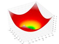
|
[math]\displaystyle{ f(\boldsymbol{x}) = \sum_{i=1}^{n} x_{i}^{2} }[/math] | [math]\displaystyle{ f(x_{1}, \dots, x_{n}) = f(0, \dots, 0) = 0 }[/math] | [math]\displaystyle{ -\infty \le x_{i} \le \infty }[/math], [math]\displaystyle{ 1 \le i \le n }[/math] |
| Функция Розенброка | 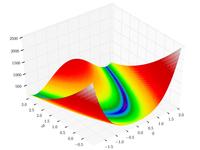
|
[math]\displaystyle{ f(\boldsymbol{x}) = \sum_{i=1}^{n-1} \left[ 100 \left(x_{i+1} - x_{i}^{2}\right)^{2} + \left(x_{i} - 1\right)^{2}\right] }[/math] | [math]\displaystyle{ \text{Min} = \begin{cases} n=2 & \rightarrow \quad f(1,1) = 0, \\ n=3 & \rightarrow \quad f(1,1,1) = 0, \\ n\gt 3 & \rightarrow \quad f(\underbrace{1,\dots,1}_{n \text{ times}}) = 0 \\ \end{cases} }[/math] | [math]\displaystyle{ -\infty \le x_{i} \le \infty }[/math], [math]\displaystyle{ 1 \le i \le n }[/math] |
| Функция Била | 
|
[math]\displaystyle{ f(x,y) = \left( 1.5 - x + xy \right)^{2} + \left( 2.25 - x + xy^{2}\right)^{2} }[/math]
[math]\displaystyle{ + \left(2.625 - x+ xy^{3}\right)^{2} }[/math] |
[math]\displaystyle{ f(3, 0.5) = 0 }[/math] | [math]\displaystyle{ -4.5 \le x,y \le 4.5 }[/math] |
| Функция Гольдшейна-Прайса | 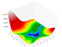
|
[math]\displaystyle{ f(x,y) = \left[1+\left(x+y+1\right)^{2}\left(19-14x+3x^{2}-14y+6xy+3y^{2}\right)\right] }[/math]
[math]\displaystyle{ \left[30+\left(2x-3y\right)^{2}\left(18-32x+12x^{2}+48y-36xy+27y^{2}\right)\right] }[/math] |
[math]\displaystyle{ f(0, -1) = 3 }[/math] | [math]\displaystyle{ -2 \le x,y \le 2 }[/math] |
| Функция Бута | 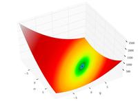
|
[math]\displaystyle{ f(x,y) = \left( x + 2y -7\right)^{2} + \left(2x +y - 5\right)^{2} }[/math] | [math]\displaystyle{ f(1,3) = 0 }[/math] | [math]\displaystyle{ -10 \le x,y \le 10 }[/math] |
| Функция Букина N 6 | 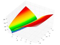
|
[math]\displaystyle{ f(x,y) = 100\sqrt{\left|y - 0.01x^{2}\right|} + 0.01 \left|x+10 \right|.\quad }[/math] | [math]\displaystyle{ f(-10,1) = 0 }[/math] | [math]\displaystyle{ -15\le x \le -5 }[/math], [math]\displaystyle{ -3\le y \le 3 }[/math] |
| Функция Матьяса | 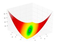
|
[math]\displaystyle{ f(x,y) = 0.26 \left( x^{2} + y^{2}\right) - 0.48 xy }[/math] | [math]\displaystyle{ f(0,0) = 0 }[/math] | [math]\displaystyle{ -10\le x,y \le 10 }[/math] |
| Функция Леви N 13 | 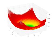
|
[math]\displaystyle{ f(x,y) = \sin^{2} 3\pi x + \left(x-1\right)^{2}\left(1+\sin^{2} 3\pi y\right) }[/math]
[math]\displaystyle{ +\left(y-1\right)^{2}\left(1+\sin^{2} 2\pi y\right) }[/math] |
[math]\displaystyle{ f(1,1) = 0 }[/math] | [math]\displaystyle{ -10\le x,y \le 10 }[/math] |
| Функция Химмельблау | 
|
[math]\displaystyle{ f(x, y) = (x^2+y-11)^2 + (x+y^2-7)^2.\quad }[/math] | [math]\displaystyle{ \text{Min} = \begin{cases} f\left(3.0, 2.0\right) & = 0.0 \\ f\left(-2.805118, 3.131312\right) & = 0.0 \\ f\left(-3.779310, -3.283186\right) & = 0.0 \\ f\left(3.584428, -1.848126\right) & = 0.0 \\ \end{cases} }[/math] | [math]\displaystyle{ -5\le x,y \le 5 }[/math] |
| Функция трехгорбого верблюда | 
|
[math]\displaystyle{ f(x,y) = 2x^{2} - 1.05x^{4} + \frac{x^{6}}{6} + xy + y^{2} }[/math] | [math]\displaystyle{ f(0,0) = 0 }[/math] | [math]\displaystyle{ -5\le x,y \le 5 }[/math] |
| Функция Изома | 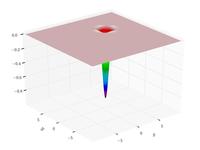
|
[math]\displaystyle{ f(x,y) = -\cos \left(x\right)\cos \left(y\right) \exp\left(-\left(\left(x-\pi\right)^{2} + \left(y-\pi\right)^{2}\right)\right) }[/math] | [math]\displaystyle{ f(\pi , \pi) = -1 }[/math] | [math]\displaystyle{ -100\le x,y \le 100 }[/math] |
| Функция "крест на подносе"
(Cross-in-tray function) |
|
[math]\displaystyle{ f(x,y) = -0.0001 \left[ \left| \sin x \sin y \exp \left(\left|100 - \frac{\sqrt{x^{2} + y^{2}}}{\pi} \right|\right)\right| + 1 \right]^{0.1} }[/math] | [math]\displaystyle{ \text{Min} = \begin{cases} f\left(1.34941, -1.34941\right) & = -2.06261 \\ f\left(1.34941, 1.34941\right) & = -2.06261 \\ f\left(-1.34941, 1.34941\right) & = -2.06261 \\ f\left(-1.34941,-1.34941\right) & = -2.06261 \\ \end{cases} }[/math] | [math]\displaystyle{ -10\le x,y \le 10 }[/math] |
| Функция "подставка для яиц"
(Eggholder function) |
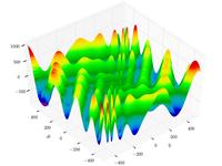
|
[math]\displaystyle{ f(x,y) = - \left(y+47\right) \sin \sqrt{\left|\frac{x}{2}+\left(y+47\right)\right|} - x \sin \sqrt{\left|x - \left(y + 47 \right)\right|} }[/math] | [math]\displaystyle{ f(512, 404.2319) = -959.6407 }[/math] | [math]\displaystyle{ -512\le x,y \le 512 }[/math] |
| Табличная функция Хольдера | 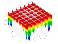
|
[math]\displaystyle{ f(x,y) = - \left|\sin x \cos y \exp \left(\left|1 - \frac{\sqrt{x^{2} + y^{2}}}{\pi} \right|\right)\right| }[/math] | [math]\displaystyle{ \text{Min} = \begin{cases} f\left(8.05502, 9.66459\right) & = -19.2085 \\ f\left(-8.05502, 9.66459\right) & = -19.2085 \\ f\left(8.05502,-9.66459\right) & = -19.2085 \\ f\left(-8.05502,-9.66459\right) & = -19.2085 \end{cases} }[/math] | [math]\displaystyle{ -10\le x,y \le 10 }[/math] |
| Функция МакКормика | 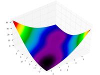
|
[math]\displaystyle{ f(x,y) = \sin \left(x+y\right) + \left(x-y\right)^{2} - 1.5x + 2.5y + 1 }[/math] | [math]\displaystyle{ f(-0.54719,-1.54719) = -1.9133 }[/math] | [math]\displaystyle{ -1.5\le x \le 4 }[/math], [math]\displaystyle{ -3\le y \le 4 }[/math] |
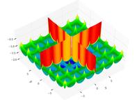
| Функция Шаффера N2 | 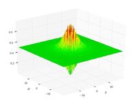
|
[math]\displaystyle{ f(x,y) = 0.5 + \frac{\sin^{2}\left(x^{2} - y^{2}\right) - 0.5}{\left[1 + 0.001\left(x^{2} + y^{2}\right) \right]^{2}} }[/math] | [math]\displaystyle{ f(0, 0) = 0 }[/math] | [math]\displaystyle{ -100\le x,y \le 100 }[/math] |
| Функция Шаффера N4 | 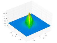
|
[math]\displaystyle{ f(x,y) = 0.5 + \frac{\cos^{2}\left[\sin \left( \left|x^{2} - y^{2}\right|\right)\right] - 0.5}{\left[1 + 0.001\left(x^{2} + y^{2}\right) \right]^{2}} }[/math] | [math]\displaystyle{ f(0,1.25313) = 0.292579 }[/math] | [math]\displaystyle{ -100\le x,y \le 100 }[/math] |
| Функция Стыбинского-Танга | 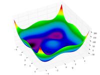
|
[math]\displaystyle{ f(\boldsymbol{x}) = \frac{\sum_{i=1}^{n} x_{i}^{4} - 16x_{i}^{2} + 5x_{i}}{2} }[/math] | [math]\displaystyle{ -39.16617n \lt f(\underbrace{-2.903534, \ldots, -2.903534}_{n \text{ times}} ) \lt -39.16616n }[/math] | [math]\displaystyle{ -5\le x_{i} \le 5 }[/math], [math]\displaystyle{ 1\le i \le n }[/math].. |
Тестовые функции для условной оптимизации
| Название | Рисунок | Формула | Глобальный минимум | Метод поиска |
|---|---|---|---|---|
| функция розенброка, ограничена кубической и прямой[1] | 
|
[math]\displaystyle{ f(x,y) = (1-x)^2 + 100(y-x^2)^2 }[/math],
subjected to: [math]\displaystyle{ (x-1)^3 - y + 1 \lt 0 \text{ and } x + y - 2 \lt 0 }[/math] |
[math]\displaystyle{ f(1.0,1.0) = 0 }[/math] | [math]\displaystyle{ -1.5\le x \le 1.5 }[/math], [math]\displaystyle{ -0.5\le y \le 2.5 }[/math] |
| Функция Розенброка, ограниченная диском[2] | 
|
[math]\displaystyle{ f(x,y) = (1-x)^2 + 100(y-x^2)^2 }[/math],
subjected to: [math]\displaystyle{ x^2 + y^2 \lt 2 }[/math] |
[math]\displaystyle{ f(1.0,1.0) = 0 }[/math] | [math]\displaystyle{ -1.5\le x \le 1.5 }[/math], [math]\displaystyle{ -1.5\le y \le 1.5 }[/math] |
| Ограниченная функция Мишры-Бёрда[3][4] | 
|
[math]\displaystyle{ f(x,y) = \sin(y) e^{\left [(1-\cos x)^2\right]} + \cos(x) e^{\left [(1-\sin y)^2 \right]} + (x-y)^2 }[/math],
subjected to: [math]\displaystyle{ (x+5)^2 + (y+5)^2 \lt 25 }[/math] |
[math]\displaystyle{ f(-3.1302468,-1.5821422) = -106.7645367 }[/math] | [math]\displaystyle{ -10\le x \le 0 }[/math], [math]\displaystyle{ -6.5\le y \le 0 }[/math] |
| Модифицированная функция Таусенда[5] | 
|
[math]\displaystyle{ f(x,y) = -[\cos((x-0.1)y)]^2 - x \sin(3x+y) }[/math],
subjected to:[math]\displaystyle{ x^2+y^2 \lt \left[2\cos t - \frac 1 2 \cos 2t - \frac 1 4 \cos 3t - \frac 1 8 \cos 4t\right]^2 + [2\sin t]^2 }[/math] where: t = Atan2(x,y) |
[math]\displaystyle{ f(2.0052938,1.1944509) = -2.0239884 }[/math] | [math]\displaystyle{ -2.25\le x \le 2.5 }[/math], [math]\displaystyle{ -2.5\le y \le 1.75 }[/math] |
| Функция Симонескуn[6] | 
|
[math]\displaystyle{ f(x,y) = 0.1xy }[/math],
subjected to: [math]\displaystyle{ x^2+y^2\le\left[r_{T}+r_{S}\cos\left(n \arctan \frac{x}{y} \right)\right]^2 }[/math] [math]\displaystyle{ \text{where: } r_{T}=1, r_{S}=0.2 \text{ and } n = 8 }[/math] |
[math]\displaystyle{ f(\pm 0.85586214,\mp 0.85586214) = -0.072625 }[/math] | [math]\displaystyle{ -1.25\le x,y \le 1.25 }[/math] |
Тестовые функции для многокритериальной оптимизации
| Название / Рисунок | Формула | Минимум | Область поиска |
|---|---|---|---|
Функция Бина и Корна 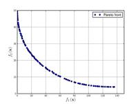
|
[math]\displaystyle{ \text{Minimize} = \begin{cases} f_{1}\left(x,y\right) & = 4x^{2} + 4y^{2} \\ f_{2}\left(x,y\right) & = \left(x - 5\right)^{2} + \left(y - 5\right)^{2} \\ \end{cases} }[/math] | [math]\displaystyle{ \text{s.t.} = \begin{cases} g_{1}\left(x,y\right) & = \left(x - 5\right)^{2} + y^{2} \leq 25 \\ g_{2}\left(x,y\right) & = \left(x - 8\right)^{2} + \left(y + 3\right)^{2} \geq 7.7 \\ \end{cases} }[/math] | [math]\displaystyle{ 0\le x \le 5 }[/math], [math]\displaystyle{ 0\le y \le 3 }[/math] |
Chakong and Haimes function 
|
[math]\displaystyle{ \text{Minimize} = \begin{cases} f_{1}\left(x,y\right) & = 2 + \left(x-2\right)^{2} + \left(y-1\right)^{2} \\ f_{2}\left(x,y\right) & = 9x - \left(y - 1\right)^{2} \\ \end{cases} }[/math] | [math]\displaystyle{ \text{s.t.} = \begin{cases} g_{1}\left(x,y\right) & = x^{2} + y^{2} \leq 225 \\ g_{2}\left(x,y\right) & = x - 3y + 10 \leq 0 \\ \end{cases} }[/math] | [math]\displaystyle{ -20\le x,y \le 20 }[/math] |
Функция Фонсеки и Флеминга 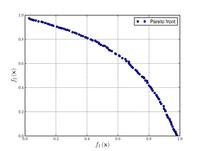
|
[math]\displaystyle{ \text{Minimize} = \begin{cases} f_{1}\left(\boldsymbol{x}\right) & = 1 - \exp \left(-\sum_{i=1}^{n} \left(x_{i} - \frac{1}{\sqrt{n}} \right)^{2} \right) \\ f_{2}\left(\boldsymbol{x}\right) & = 1 - \exp \left(-\sum_{i=1}^{n} \left(x_{i} + \frac{1}{\sqrt{n}} \right)^{2} \right) \\ \end{cases} }[/math] | [math]\displaystyle{ -4\le x_{i} \le 4 }[/math], [math]\displaystyle{ 1\le i \le n }[/math] | |
Test function 4 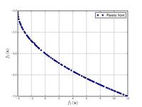
|
[math]\displaystyle{ \text{Minimize} = \begin{cases} f_{1}\left(x,y\right) & = x^{2} - y \\ f_{2}\left(x,y\right) & = -0.5x - y - 1 \\ \end{cases} }[/math] | [math]\displaystyle{ \text{s.t.} = \begin{cases} g_{1}\left(x,y\right) & = 6.5 - \frac{x}{6} - y \geq 0 \\ g_{2}\left(x,y\right) & = 7.5 - 0.5x - y \geq 0 \\ g_{3}\left(x,y\right) & = 30 - 5x - y \geq 0 \\ \end{cases} }[/math] | [math]\displaystyle{ -7\le x,y \le 4 }[/math] |
Функция Курсаве 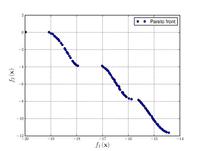
|
[math]\displaystyle{ \text{Minimize} = \begin{cases} f_{1}\left(\boldsymbol{x}\right) & = \sum_{i=1}^{2} \left[-10 \exp \left(-0.2 \sqrt{x_{i}^{2} + x_{i+1}^{2}} \right) \right] \\ & \\ f_{2}\left(\boldsymbol{x}\right) & = \sum_{i=1}^{3} \left[\left|x_{i}\right|^{0.8} + 5 \sin \left(x_{i}^{3} \right) \right] \\ \end{cases} }[/math] | [math]\displaystyle{ -5\le x_{i} \le 5 }[/math], [math]\displaystyle{ 1\le i \le 3 }[/math]. | |
Schaffer function N. 1 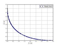
|
[math]\displaystyle{ \text{Minimize} = \begin{cases} f_{1}\left(x\right) & = x^{2} \\ f_{2}\left(x\right) & = \left(x-2\right)^{2} \\ \end{cases} }[/math] | [math]\displaystyle{ -A\le x \le A }[/math]. Values of [math]\displaystyle{ A }[/math] form [math]\displaystyle{ 10 }[/math] to [math]\displaystyle{ 10^{5} }[/math] have been used successfully. Higher values of [math]\displaystyle{ A }[/math] increase the difficulty of the problem. | |
Schaffer function N. 2 
|
[math]\displaystyle{ \text{Minimize} = \begin{cases} f_{1}\left(x\right) & = \begin{cases} -x, & \text{if } x \le 1 \\ x-2, & \text{if } 1 \lt x \le 3 \\ 4-x, & \text{if } 3 \lt x \le 4 \\ x-4, & \text{if } x \gt 4 \\ \end{cases} \\ f_{2}\left(x\right) & = \left(x-5\right)^{2} \\ \end{cases} }[/math] | [math]\displaystyle{ -5\le x \le 10 }[/math]. | |
Объективная функция Полони2 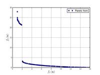
|
[math]\displaystyle{ \text{Minimize} =
\begin{cases}
f_{1}\left(x,y\right) & = \left[1 + \left(A_{1} - B_{1}\left(x,y\right) \right)^{2} + \left(A_{2} - B_{2}\left(x,y\right) \right)^{2} \right] \\
f_{2}\left(x,y\right) & = \left(x + 3\right)^{2} + \left(y + 1 \right)^{2} \\
\end{cases}
}[/math]
[math]\displaystyle{ \text{where} = \begin{cases} A_{1} & = 0.5 \sin \left(1\right) - 2 \cos \left(1\right) + \sin \left(2\right) - 1.5 \cos \left(2\right) \\ A_{2} & = 1.5 \sin \left(1\right) - \cos \left(1\right) + 2 \sin \left(2\right) - 0.5 \cos \left(2\right) \\ B_{1}\left(x,y\right) & = 0.5 \sin \left(x\right) - 2 \cos \left(x\right) + \sin \left(y\right) - 1.5 \cos \left(y\right) \\ B_{2}\left(x,y\right) & = 1.5 \sin \left(x\right) - \cos \left(x\right) + 2 \sin \left(y\right) - 0.5 \cos \left(y\right) \end{cases} }[/math] |
[math]\displaystyle{ -\pi\le x,y \le \pi }[/math] | |
Функция Зистера-Дьеба-Тери N. 1 
|
[math]\displaystyle{ \text{Minimize} = \begin{cases} f_{1}\left(\boldsymbol{x}\right) & = x_{1} \\ f_{2}\left(\boldsymbol{x}\right) & = g\left(\boldsymbol{x}\right) h \left(f_{1}\left(\boldsymbol{x}\right),g\left(\boldsymbol{x}\right)\right) \\ g\left(\boldsymbol{x}\right) & = 1 + \frac{9}{29} \sum_{i=2}^{30} x_{i} \\ h \left(f_{1}\left(\boldsymbol{x}\right),g\left(\boldsymbol{x}\right)\right) & = 1 - \sqrt{\frac{f_{1}\left(\boldsymbol{x}\right)}{g\left(\boldsymbol{x}\right)}} \\ \end{cases} }[/math] | [math]\displaystyle{ 0\le x_{i} \le 1 }[/math], [math]\displaystyle{ 1\le i \le 30 }[/math]. | |
Функция Зистера-Дьеба-Тери N. 2 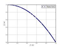
|
[math]\displaystyle{ \text{Minimize} = \begin{cases} f_{1}\left(\boldsymbol{x}\right) & = x_{1} \\ f_{2}\left(\boldsymbol{x}\right) & = g\left(\boldsymbol{x}\right) h \left(f_{1}\left(\boldsymbol{x}\right),g\left(\boldsymbol{x}\right)\right) \\ g\left(\boldsymbol{x}\right) & = 1 + \frac{9}{29} \sum_{i=2}^{30} x_{i} \\ h \left(f_{1}\left(\boldsymbol{x}\right),g\left(\boldsymbol{x}\right)\right) & = 1 - \left(\frac{f_{1}\left(\boldsymbol{x}\right)}{g\left(\boldsymbol{x}\right)}\right)^{2} \\ \end{cases} }[/math] | [math]\displaystyle{ 0\le x_{i} \le 1 }[/math], [math]\displaystyle{ 1\le i \le 30 }[/math]. | |
Функция Зистера-Дьеба-Териn N. 3 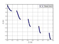
|
[math]\displaystyle{ \text{Minimize} = \begin{cases} f_{1}\left(\boldsymbol{x}\right) & = x_{1} \\ f_{2}\left(\boldsymbol{x}\right) & = g\left(\boldsymbol{x}\right) h \left(f_{1}\left(\boldsymbol{x}\right),g\left(\boldsymbol{x}\right)\right) \\ g\left(\boldsymbol{x}\right) & = 1 + \frac{9}{29} \sum_{i=2}^{30} x_{i} \\ h \left(f_{1}\left(\boldsymbol{x}\right),g\left(\boldsymbol{x}\right)\right) & = 1 - \sqrt{\frac{f_{1}\left(\boldsymbol{x}\right)}{g\left(\boldsymbol{x} \right)}} - \left(\frac{f_{1}\left(\boldsymbol{x}\right)}{g\left(\boldsymbol{x}\right)} \right) \sin \left(10 \pi f_{1} \left(\boldsymbol{x} \right) \right) \end{cases} }[/math] | [math]\displaystyle{ 0\le x_{i} \le 1 }[/math], [math]\displaystyle{ 1\le i \le 30 }[/math]. | |
Функция Зистера-Дьеба-ТериN. 4 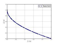
|
[math]\displaystyle{ \text{Minimize} = \begin{cases} f_{1}\left(\boldsymbol{x}\right) & = x_{1} \\ f_{2}\left(\boldsymbol{x}\right) & = g\left(\boldsymbol{x}\right) h \left(f_{1}\left(\boldsymbol{x}\right),g\left(\boldsymbol{x}\right)\right) \\ g\left(\boldsymbol{x}\right) & = 91 + \sum_{i=2}^{10} \left(x_{i}^{2} - 10 \cos \left(4 \pi x_{i}\right) \right) \\ h \left(f_{1}\left(\boldsymbol{x}\right),g\left(\boldsymbol{x}\right)\right) & = 1 - \sqrt{\frac{f_{1}\left(\boldsymbol{x}\right)}{g\left(\boldsymbol{x} \right)}} \end{cases} }[/math] | [math]\displaystyle{ 0\le x_{1} \le 1 }[/math], [math]\displaystyle{ -5\le x_{i} \le 5 }[/math], [math]\displaystyle{ 2\le i \le 10 }[/math] | |
Функция Зистера-Дьеба-Тери N. 6 
|
[math]\displaystyle{ \text{Minimize} = \begin{cases} f_{1}\left(\boldsymbol{x}\right) & = 1 - \exp \left(-4x_{1}\right)\sin^{6}\left(6 \pi x_{1} \right) \\ f_{2}\left(\boldsymbol{x}\right) & = g\left(\boldsymbol{x}\right) h \left(f_{1}\left(\boldsymbol{x}\right),g\left(\boldsymbol{x}\right)\right) \\ g\left(\boldsymbol{x}\right) & = 1 + 9 \left[\frac{\sum_{i=2}^{10} x_{i}}{9}\right]^{0.25} \\ h \left(f_{1}\left(\boldsymbol{x}\right),g\left(\boldsymbol{x}\right)\right) & = 1 - \left(\frac{f_{1}\left(\boldsymbol{x}\right)}{g\left(\boldsymbol{x} \right)}\right)^{2} \\ \end{cases} }[/math] | [math]\displaystyle{ 0\le x_{i} \le 1 }[/math], [math]\displaystyle{ 1\le i \le 10 }[/math]. | |
Функция Виннета 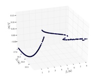
|
[math]\displaystyle{ \text{Minimize} = \begin{cases} f_{1}\left(x,y\right) & = 0.5\left(x^{2} + y^{2}\right) + \sin\left(x^{2} + y^{2} \right) \\ f_{2}\left(x,y\right) & = \frac{\left(3x - 2y + 4\right)^{2}}{8} + \frac{\left(x - y + 1\right)^{2}}{27} + 15 \\ f_{3}\left(x,y\right) & = \frac{1}{x^{2} + y^{2} + 1} - 1.1 \exp \left(- \left(x^{2} + y^{2} \right) \right) \\ \end{cases} }[/math] | [math]\displaystyle{ -3\le x,y \le 3 }[/math]. | |
Функция Осызки и Кунду 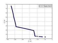
|
[math]\displaystyle{ F_{1}(x) = -25 \left(x_{1}-2\right)^{2} - \left(x_{2}-2\right)^{2} }[/math]
[math]\displaystyle{ - \left(x_{3}-1\right)^{2} - \left(x_{4}-4\right)^{2} - \left(x_{5}-1\right)^{2} }[/math] |
[math]\displaystyle{ \text{s.t.} = \begin{cases} g_{1}\left(\boldsymbol{x}\right) & = x_{1} + x_{2} - 2 \geq 0 \\ g_{2}\left(\boldsymbol{x}\right) & = 6 - x_{1} - x_{2} \geq 0 \\ g_{3}\left(\boldsymbol{x}\right) & = 2 - x_{2} + x_{1} \geq 0 \\ g_{4}\left(\boldsymbol{x}\right) & = 2 - x_{1} + 3x_{2} \geq 0 \\ g_{5}\left(\boldsymbol{x}\right) & = 4 - \left(x_{3}-3\right)^{2} - x_{4} \geq 0 \\ g_{6}\left(\boldsymbol{x}\right) & = \left(x_{5} - 3\right)^{2} + x_{6} - 4 \geq 0 \end{cases} }[/math] | [math]\displaystyle{ 0\le x_{1},x_{2},x_{6} \le 10 }[/math], [math]\displaystyle{ 1\le x_{3},x_{5} \le 5 }[/math], [math]\displaystyle{ 0\le x_{4} \le 6 }[/math]. |
CTP1 function (2 variables) 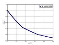
|
[math]\displaystyle{ \text{Minimize} = \begin{cases} f_{1}\left(x,y\right) & = x \\ f_{2}\left(x,y\right) & = \left(1 + y\right) \exp \left(-\frac{x}{1+y} \right) \end{cases} }[/math] | [math]\displaystyle{ \text{s.t.} = \begin{cases} g_{1}\left(x,y\right) & = \frac{f_{2}\left(x,y\right)}{0.858 \exp \left(-0.541 f_{1}\left(x,y\right)\right)} \geq 1 \\ g_{1}\left(x,y\right) & = \frac{f_{2}\left(x,y\right)}{0.728 \exp \left(-0.295 f_{1}\left(x,y\right)\right)} \geq 1 \end{cases} }[/math] | [math]\displaystyle{ 0\le x,y \le 1 }[/math]. |
Проблема Констр-Экса 
|
[math]\displaystyle{ \text{Minimize} = \begin{cases} f_{1}\left(x,y\right) & = x \\ f_{2}\left(x,y\right) & = \frac{1 + y}{x} \\ \end{cases} }[/math] | [math]\displaystyle{ \text{s.t.} = \begin{cases} g_{1}\left(x,y\right) & = y + 9x \geq 6 \\ g_{1}\left(x,y\right) & = -y + 9x \geq 1 \\ \end{cases} }[/math] | [math]\displaystyle{ 0.1\le x \le 1 }[/math], [math]\displaystyle{ 0\le y \le 5 }[/math] |
См. также
Литература
- Пантелеев А. В., Метлицкая Д. В., Е.А. Алешина Методы глобальной оптимизации. Метаэвристические стратегии и алгоритмы // М.: Вузовская книга. 2013. 244 с. ISBN 978-5-9502-0743-3
- Сергиенко А. Б. Тестовые функции для глобальной оптимизации.
Ссылки
Примечания
- ↑ Simionescu, P.A. New Concepts in Graphic Visualization of Objective Functions // (ASME 2002 International Design Engineering Technical Conferences and Computers and Information in Engineering Conference). — Montreal, Canada. — P. 891–897.
- ↑ Solve a Constrained Nonlinear Problem - MATLAB & Simulink. www.mathworks.com. Дата обращения: 29 августа 2017. Архивировано 29 августа 2017 года.
- ↑ Bird Problem (Constrained) | Phoenix Integration (недоступная ссылка). wayback.archive.org. Дата обращения: 29 августа 2017. Архивировано 29 декабря 2016 года.
- ↑ Mishra, Sudhanshu. Some new test functions for global optimization and performance of repulsive particle swarm method (англ.) // MPRA Paper : journal. — 2006. Архивировано 4 ноября 2018 года.
- ↑ Townsend, Alex Constrained optimization in Chebfun. chebfun.org (январь 2014). Дата обращения: 29 августа 2017. Архивировано 29 августа 2017 года.
- ↑ Simionescu, P.A. Computer Aided Graphing and Simulation Tools for AutoCAD Users (англ.). — 1st. — Boca Raton, FL: CRC Press, 2014. — ISBN 978-1-4822-5290-3.